How to copy charts into a word processor

When copying charts into a word processor, whether in Microsoft Office from Excel to Word or in openoffice.org from Calc to Writer, the software embeds a special object that links back to the original spreadsheet. If you then change the details in the Excel spreadsheet the chart in the Word document will change accordingly. In many cases this is advantageous; however, it can cause problems if the Word document cannot 'see' the Excel file, for example, if you email the Word file to someone without the Excel file. It is generally better to paste the chart as an image in the first place using the 'Paste special' facility.

I will start by explaining how to do this in Microsoft Office:

Once you have created your chart in Excel you select it and copy it, as shown here.


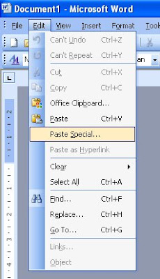
In older versions of Word you pull down the 'Edit' menu and select 'Paste Special'. You may have to wait a moment for all the menu items to be revealed.


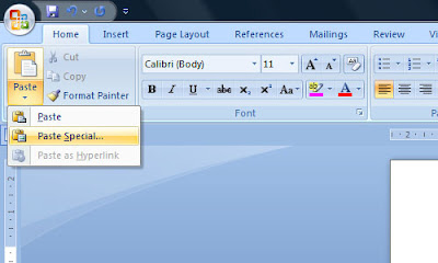
In the latest versions of Word, 'Paste special' is in a menu underneath the 'Paste' button.


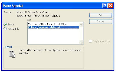
A box will open, from which you select 'Picture (Enhanced Metafile)', and click OK.

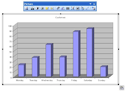
This will then insert the chart as a picture, which you can manipulate like any other imported image.
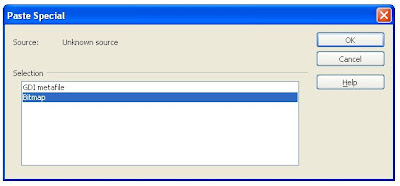
In openoffice.org, the procedure is pretty much the same as above, with 'Paste special' is in the 'Edit' menu, or alternatively you can use a keyboard shortcut: Ctrl + Shift + V. The major difference from above is that the following box will open when you select 'Paste special'. Simply select 'Bitmap' and click OK to paste the chart as a picture.

Read More

Adding custom lists to Excel and OpenOffice.org

In the last post I demonstrated how to easily enter lists of numbers, days of the week and months of the year in Excel and Calc (the OpenOffice.org spreadsheet application). Both programs offer the option to add custom lists to this feature. In this post I will show you how to add the colours of the spectrum as a new list.

Excel 2003 and earlier
Open up Excel and type the colours of the rainbow into one of the columns, then select the cells as shown below.

Pull down the 'Tools' menu and select 'Options', then go to the 'Custom Lists' tab.

You should see an entry in the 'Import list from cells' box. Click on the 'Import' button to the right of this to add the list.

The colours list will appear in the 'List entries' box. Rather than type the entries into cells, you could just type the list in this box, pressing Enter after each item, and then click the 'Add' button to save the list.

Click 'OK', and the list is available to use. Simply type 'Red' in a cell and drag the handler down to automatically fill consecutive cells with the other colours.


Excel 2007 and later
Follow the previous instructions, except to open the 'Options' box click the Microsoft Office Button (shown right), and then click the 'Excel Options' button.

On the 'Popular' page, click the 'Edit Custom Lists' button and continue as above.

OpenOffice.org Calc

Type the list of colours into a column of cells and select them as shown.

From the 'Tools' menu, select 'Options', then click the + next to 'OpenOffice.org calc' in the list, to expand its entries, then click on 'Sort Lists', as shown.

You should see an entry in the 'Copy list from' box. Click on the 'Copy' button to the right of this to add the list.

Click 'OK', and the list is available to use.

As with Excel, you can enter a list manually by clicking the 'New' button on the 'Sort Lists' option box, typing in the entries, and then pressing the 'Add' button.

Read More

How to quickly enter lists in Excel and OpenOffice

Excel spreadsheets often have a column or a row of incremental data. That is, information in the form of a list of numbers (1, 2, 3, 4, etc), times (09:00, 10:00, 11:00, etc), the names of months or the days of the week. You could type all this information into the row or column yourself, or you can let Excel handle it for you.

To try this out open Excel and type 1 in any cell, and 2 in the cell below it. For lists of numbers you need to enter a couple of numbers so that Excel knows where to begin and what interval to use.

Select both the cells (by hovering the mouse pointer over the top of one, holding down the left button, moving to the other cell and letting go).

You will notice that there is a small square in the bottom right hand corner of the selection box. If you hover the mouse pointer over this square the pointer will change to a + symbol. If you hold down the left mouse button and drag downwards Excel will fill in the cells continuing the series of numbers.

You can do the same with larger increments too. The images to the left show the same process being used to generate is a list of numbers with an interval of 10.

But that is far from all you can do with this process. You can drag these lists in any direction so that you can create rows as well as columns. Also, you are not limited to numbers; you can produce lists of months, days of the week, and times. I have included a video in this post showing this feature of Excel in action creating a few of these lists.

Calc, the OpenOffice spreadsheet package, works in pretty much the same way, except that there are no default intervals for times. So, if you enter 00:00 and drag the handler down selecting consecutive cells they will all also be filled with 00:00, but this is easily solved by entering 00:00 in the first cell and 01:00 in the second, then selecting both cells and dragging the handler down.

In the next post I will show you how to set up your own custom lists in Excel and Calc.

Read More

Customising the Quick Access Toolbar

In a recent post about adding buttons to the toolbars in Microsoft Office applications I pointed out that there is no way to add buttons to the new 'ribbon' that has replaced the old toolbars. Nevertheless, it has come to my attention that there is still one customisable toolbar in the latest versions of Word, Excel and Powerpoint. This is called the 'Quick Access Toolbar'. If you wish to add extra buttons to this toolbar you can do so by following the instructions on the 'Microsoft Office Online' pages. [http://office.microsoft.com/en-us/word/HA012341051033.aspx]

I do not have a copy of MS Office 2007 myself, so I do not know whether you can add a button for the useful 'Past Special' function. If you have a copy of any of the Office 2007 applications, please let me know how you have got on when adding buttons to this toolbar.

Read More

Printing from Excel - Part 2

In the last post I showed how to format an Excel sheet so that it fitted to the page and added page numbers. The end result as displayed in Print Preview is as shown here.


As we can see there are no gridlines on the print. We can either remedy this by selecting border types on the table or, more easily, we can set a print option to show simple gridlines. To do this go to Print Preview, click the 'Setup...' button and select the 'Sheet' tab. Here, I select the Print Gridlines option, as shown.


After I click 'OK', the Print Preview looks like this. I have zoomed in on the preview so that you can see the gridlines more clearly.


The above is a preview of page 2, where we can see that there are no column headers as there are on page 1. We can tell Excel to print the column headers on each page to make the print of the table more user-friendly. To do this I need to close the Print Preview, and select 'Page Setup' from the 'File' menu, which enables some extra options. On the 'Sheet' tab I click the circled button.


This opens the following option box. I now click the row that I want to repeat. In this case it is row 1, so I click the appropriate button as circled in red, and close the option box by clicking the button circled in green. This will enter the appropriate code into the 'Rows to repeat at top' option. After, I click 'OK' I have a well formatted spreadsheet ready to be printed.


As you can see there are a number of other options that I have not explored here. If you have a document that prints on many pages you may want to click the 'Margins' button and adjust the size of the print area by clicking and dragging the various dotted lines, but be careful to leave enough of a margin around the table so that the print is not ruined - at least a centimetre (or about half an inch) should be enough. If you have a particularly wide document you may not be able to fit it onto one page width, in which case you can also set the print to repeat columns in much the same way as I did for rows. Printing Excel spreadsheets may be a fiddly business, but with a little effort you can achieve some very good results.

Read More

Printing from Excel - Part 1

Printing from Microsoft Excel is markedly different to printing from Word. Whereas in Word we can usually just tell it to print without worrying that much about formatting the page, in Excel we will usually have to specifically tell it how we want to print our speadsheets, and this can sometimes be a little fiddly. Because there is quite a lot of fiddling that can be done I have split these instructions over two posts.


Pictured above is an example of a spreadsheet - in this case a dataset of U.S. population information. Exciting, I know. When I press the Print Preview button [pictured right] I see the following:


As we can see, not all the columns are shown on the first page. If I go down to page 6 we can see the missing column.


To remedy this situation I click the 'Setup..' button in the Print Preview. This opens up the following option box.


I could change the orientation to 'Landscape' as this would enable the missing column ; however, for the purposes of this tutorial I will keep it set to 'Portrait'. Instead, I reduce the scaling until the final column appears on the first page. In this case I set it to 80% of normal size.


I could also have achieved the same result by selecting all the data and reducing the font size, the column width and row height; although I find adjusting the scaling to be easier. The Print Preview now looks like this:


As yet there are no page numbers shown. In order to have page numbers displayed I click 'Setup..' again and open the 'Header/Footer' tab. Here I can select whether I want the page numbers to be shown at the top or the bottom of the page by choosing an option from the appropriate drop-down list, two of which are shown below.


As you can see from the drop-down lists, there are other options available for what will be displayed in the header or footer, including file name and date. I now have a serviceable format for my document that I can print out. At the same time I have reduced the number of pages from ten to four. There are a number of other print formatting options available that I will explore in the next post.

Read More

Putting new buttons on toolbars in MS Office (before the 2007 version)

A while ago I published an article that suggested that rather than printing directly from web browsers, such as Internet Explorer, it is better to copy the information that you want into a word processor and print it from there. In that article I mentioned the use of the 'Paste Special' in Word, which enables you to remove formatting from the information that you paste. In this article I will explain how to put a button for 'Paste Special' onto the toolbar in Microsoft Word 2003 and other earlier versions. This technique can also be used to add any of the other available buttons onto any toolbar.

Open up Word and right-click on one of the toolbars, which are at the top of the screen below the menu and look something like this:


From the menu, select 'Customize...', which will open a dialog box. Click on the 'Commands' tab.


Select 'Edit' from the left-hand menu, because the 'Paste Special' tool is listed in the 'Edit' menu. Scroll down through the list on the right-hand until you see 'Paste Special' then left-click on it and hold the mouse button down. The mouse pointer should change to an arrow pointing at a rectangle with a square to the bottom right, which will have an X in it initially.

Move the pointer up to the toolbars and release the mouse button when it is in a suitable position: next to the normal paste button for example. You will notice that the mouse pointer changed appearance again when you hovered over the toolbar, with the X being replaced with a + to let you know that the new button can be placed there.

Your toolbar should now look something like this:

If you wish to remove a button from the toolbar, follow the instructions above for opening the 'Customize' dialog, but rather than drag from the dialog box to the toolbar, click on the button you wish to remove from the toolbar and drag it into the dialog box.

This process also works in the other Microsoft Office applications such as Excel and PowerPoint. With Office 2007, Microsoft have replaced the old tried-and-tested menu and toolbar arrangement with something called 'ribbons' (as pictured below) and there is no way to customise these in the same way as detailed above.

This is an edited version of a post that first appeared on Bloody Computer! on 19th November 2007.

Read More

How to quickly enter lists of numbers, dates and times in Excel

Excel spreadsheets often have a column or a row of incremental data. That is, information in the form of a list of numbers (1, 2, 3, 4, etc), times (09:00, 10:00, 11:00, etc), the names of months or the days of the week. You could type all this information into the row or column yourself, or you can let Excel handle it for you.

To try this out open Excel and type 1 in any cell, and 2 in the cell below it. For lists of numbers you need to enter a couple of numbers so that Excel knows where to begin and what interval to use.

Select both the cells (by hovering the mouse pointer over the top of one, holding down the left button, moving to the other cell and letting go).

You will notice that there is a small square in the bottom right hand corner of the selection box. If you hover the mouse pointer over this square the pointer will change to a + symbol. If you hold down the left mouse button and drag downwards Excel will fill in the cells continuing the series of numbers.

You can do the same with larger increments too. The images to the left show the same process being used to generate is a list of numbers with an interval of 10.

But that is far from all you can do with this process. You can drag these lists in any direction so that you can create rows as well as columns. Also, you are not limited to numbers; you can produce lists of months, days of the week, and times. I have included a video in this post showing this feature of Excel in action creating a few of these lists.

Read More

Putting new buttons on toolbars in MS Office

A while ago I wrote an article that suggested that rather than printing directly from web browsers, such as Internet Explorer, it is better to copy the information that you want into a word processor and print it from there. In that article I mentioned the use of the 'Paste Special' in Word, which enables you to remove formatting from the information that you paste. In this article I will explain how to put a button for 'Paste Special' onto the toolbar in word. This technique can also be used to add any of the other available buttons onto the toolbar.

Open up word and right-click on one of the toolbars, which are at the top of the screen below the menu and look something like this:


From the menu, select 'Customize...', which will open a dialog box. Click on the 'Commands' tab.


Select 'Edit' from the left-hand menu, because the 'Paste Special' tool is listed in the 'Edit' menu. Scroll down through the list on the right-hand until you see 'Paste Special' then left-click on it and hold the mouse button down. The mouse pointer should change to an arrow pointing at a rectangle with a square to the bottom right, which will have an X in it initially.

Move the pointer up to the toolbars and release the mouse button when it is in a suitable position: next to the normal paste button for example. You will notice that the mouse pointer changed appearance again when you hovered over the toolbar, with the X being replaced with a + to let you know that the new button can be placed there.

Your toolbar should now look something like this:

If you wish to remove a button from the toolbar, follow the instructions above for opening the 'Customize' dialog, but rather than drag from the dialog box to the toolbar, click on the button you wish to remove from the toolbar and drag it into the dialog box.

This process also works in the other Microsoft Office applications such as Excel and PowerPoint.

Read More

Keyboard shortcut of the week: search and find

If you wish to bring up Windows' file search minimise all your windows and press F3. You can also search within a certain folder too: open that folder up in Windows Explorer (the name for the program that opens when you double click on 'My Documents', 'My Computer', etc) and - you guessed it - press F3.

Pressing F3 opens search dialogs in many other programs as well: in Internet Explorer it opens (and closes) the vertical search bar; in MS Outlook it opens up the 'Advanced Find' dialog. Try pressing F3 when using applications that have some sort of search facility.

In a similar vein, you can open up the find facility in many applications by holding down the Control ('Ctrl') key and pressing F. To explain the difference between search and find, consider that you will search for a web page and when you have opened it you can find text within it. In MS Word Ctrl + F opens the 'Find and Replace' dialog. As with F3, try it out in any program that has a find facility.

Of course some programmers use slightly different standards. For example in Firefox both F3 and Ctrl + F open the find word dialog at the bottom of the screen.

Happy hunting.

Read More

Keyboard shortcut of the week: Excel

Following on from the megapost of word-processing keyboard shortcuts from earlier this month, here is a selection of keyboard shortcuts for Microsoft Excel.

• You can navigate around the grid of cells by using the cursor keys.
• Hold down Ctrl and press Home to jump to the top right cell (A1).
• Hold down Ctrl and End to jump to the last cell on the spreadsheet with any information in
  
• If you wish to edit the contents of a cell press F2
  

As with word processing, you can hold down the Shift key to select: if you hold down Shift and press the right cursor key then you will select the current cell and the one to the right of it. If you continue to hold down the Shift key and press the down cursor key you will also select the two cells below the ones you already had selected. You can thus hold down the Shift key and press different cursor keys to select different rectangles of cells.

Many of the keyboard shortcuts that work for word processing also work in Excel: holding down Ctrl and pressing B selects bold text; Ctrl and C will copy text, etc.

Read More